Tag

Showing blog posts sorted under the tag: machine learning

Detecting Northern Lights using Raspberry Pi and Convolutional Neural Network - Part 1

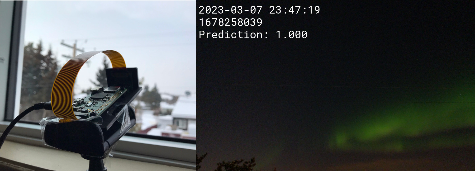
Pi Camera and a Northern Lights image with prediction.

At the moment, I'm fortunate to live in a part of the world where visible Northern Lights are fairly common. The problem is though, they may only show up for a few minutes during the night so you have to either be a real night-owl or get lucky. I wanted to build something to help me catch the Northern Lights more often.

The idea mostly came after seeing the recent release of the Raspberry Pi camera module 3 and wanting an excuse to do something with it.

In this blog post I'll go over the proof of concept of the idea and how I hope to develop the project into something a little nicer.

I already had a bit of a head-start on the some of the infrastructure from a previous project of mine, a Raspberry Pi baby monitor. It's a two-part setup a camera-equipped Pi Zero W and a separate server component running on my home server. The Pi Zero is a 'dumb' piece that only takes pictures every few seconds and sends it via http, while all the business logic of collecting, storing, and displaying pictures sits on my server. This makes it easy to unplug and move the camera around without causing too much trouble to the whole system's operation.

For this particular project, my Pi Zero got a camera 3 upgrade and was pointed straight at the sky out my north-facing, upstairs window. It captures a picture every 5 seconds and sends it to my home server where it's stored for later; most nights capturing about 7000 images. Each image is stored in a folder and metadata about the image is written to a small sqlite3 database. To label the images, I was able to use my computer's image previewer to quickly scrub through a nights worth of images and mark them in the database as either containing Northern Lights or not. It only took about 30 minutes per night but it was pretty boring work none-the-less.

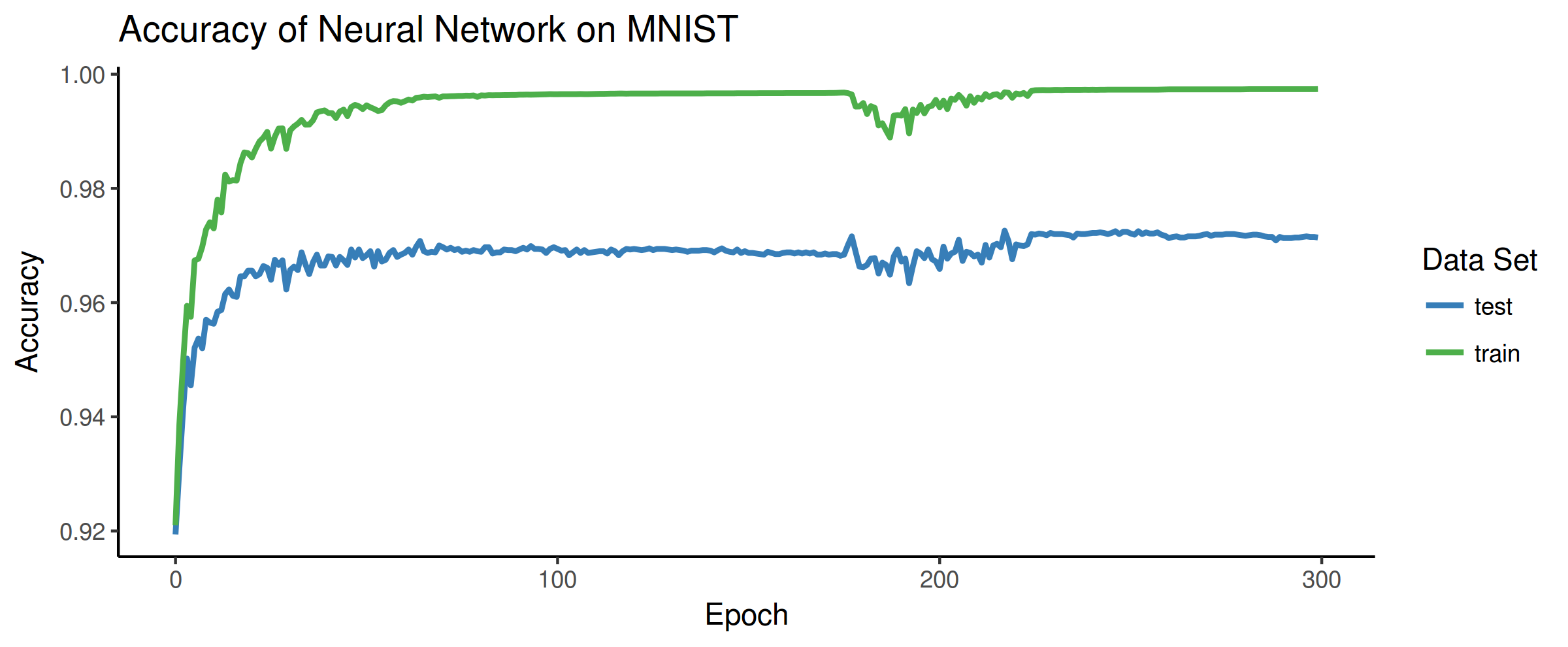
With labelled images, I could sort them into a proper training dataset of 'aurora' and 'sky' pictures. I then trained a large convolutional neural network built using the Keras Python package to classify the pictures. The Keras documentation has a nice article called 'Image Classification from Scratch' which was a good starting point for this task. It shows how to build a model to classify pictures as either dogs or cats, so it was fairly straightforward to adapt it to the task of classifying 'Aurora' or 'No Aurora'.

Below is a YouTube video showing a full night of particularly active Northern Lights. The 3rd number in the top-left of each image is the prediction from the trained neural network, the closer to 1 the number is the more confident the model is that the picture contains Northern Lights. None of the pictures in this timelapse were used in training the model. Skip ahead to 0:50 to see the Northern Lights in action!


With the concept proven, I'd like to build the whole project out a little bit more. The step 2 is to build a proper webapp that can receive pictures from the Pi, classify them, and display them. The best pictures (according the model) will get saved, and on really good nights it should send me a text message or some other notification. It will probably be a bit tricky to come up with a good heuristic for this, as sometimes Northern Lights will be gone within a few minutes.

Step 3 is to build a better enclosure for the Raspberry Pi so that I can move it outside to a more permanent location. I'm more of a software person so I haven't thought too much about this. If anybody has any god suggestions please let me know.

That's it for now. Thanks for reading. I'll try to put the code and training pictures on GitHub soon.

Update

I've been playing a bit with Google Colab and thought it would be a good way to share the training code and data for this project.

Python Notebook: https://colab.research.google.com/drive/1CFNfKZH_WyrGN71t4Jx4NU-FzBTAeZP5?usp=sharing

Training Images (1.4GB): https://drive.google.com/file/d/1N8uuIMo6AzM6SGoTBQh7iWK_SGIOyh6n/view?usp=sharing


Tags:


Neural Network from Scratch


It’s been a while since my last machine learning project: implementing a decision tree in Julia. This time I wanted to take a closer look at neural networks. I was recently shown an amazing book 'Neural Networks and Deep Learning' by Michael Nielson. He does a great job distilling the basics to a point where his explanations become intuitive. I won't be able to explain anything as well as he does so please check out his book.

The most basic neural networks are, as it turns out, surprisingly simple. It is possible to derive methods for building and training neural networks using only basic linear algebra and calculus. Neural networks have also been around for quite some time but it wasn’t until backpropagation was suggested as a way of training networks in the 70's that they really took off. The complexity of them stems somewhat from the sheer size of networks. Modern computer hardware and new scientific computing methods were required for neural networks to reach the popularity they have today.

Backpropagation is the key to training neural networks. Essentially, backpropagation takes the error at the output of a network and updates weights, within the network, based on how much they contributed to that error. By calculating the error from a sample and adjusting the weights accordingly over many, many iterations the network can be trained.

So in keeping with my previous project, I implemented a basic backpropogation algorithm in C for training on the popular MNIST dataset. I used a combination of the GNU Scientific Library and OpenBLAS for all the heavy number crunching. For the network itself I went with 2 hidden layers (4 total, including input and output layers) of 100 and 30 neurons. Below is the result after training on 50,000 images:


The green shows accuracy on training data and the blue shows the neural networks accuracy on a separate set of testing data. The x-axis shows the number of epochs, or the number of times the backpropagation went through all the training data and updated the network. Interestingly, after about 100 epochs the accuracy on the test data starts to decrease slightly. This is a sign that the network was overfitting to the training data. However, after around 180 epochs there is some disruption which ended up increasing the accuracy on both the training and testing data sets. Overall the accuracy was 99.74% and 97.14% on the training and testing data respectively.

As a final test, I got my lovely wife to draw any number on the computer (she chose '4'). I then fed this into the neural network to get see if it could identify what she wrote:


Clearly there is something to these neural networks after-all.

Thank you for reading. Please check out Michael's book if you want to know more about neural networks. Also check out the code I wrote for this network on my Github.


Tags:


Simple Regression Trees in Julia

Being a data analyst, it’s a bit embarrassing how little experience I have with the new hotness of machine learning. I recently had a conversation with an individual who mentioned that they often employ decision and regression trees as a data exploration method and this prompted me to start looking into them.

Decision and regression trees are an awesome tool because of how transparent the end result is. It’s easy to understand and to explain to others who might be weary of implementing something opaque. In the simplest trees, they ask a series of yes-no questions such as: is a certain variable greater than some number. With each question you progress through different paths until you reach a terminal node. This terminal node will give you a prediction, either a classification or a value, depending on the type of tree. This process is extremely easy to follow and is the biggest selling point of decision trees.

Another advantage of decision trees is the simplicity of the algorithm used to create the tree. There are 3 basic steps that go into creating a tree. The first is a calculation on some cost function that we want to minimize. In the case of regression trees the cost function is usually just the mean squared error of all observations at that particular node. Secondly, each variable is iterated over to find the optimal way to divide the observations into two groups. Optimal, in this case, refers to the smallest mean squared error. And finally, once the optimal division is found the process is repeated on the two subgroups. This continues until certain predefined conditions are reached like minimum number of observations at a node.

In fact, the algorithm is so simple I decided to implement a basic regression tree in Julia as a learning exercise. Julia is an awesome statistical computing language thats main advantage is speed. Code written in Julia is often several times faster than the equivalent R or Python code for non-trivial calculations. My implementation is rather limited compared to the ‘rpart’ package in R or even the ‘DecisionTrees.jl’ package available in Julia. The idea was to gain a better understanding of how decision trees actually work and not to replace any of the already great implementations available.

I tested my implementation on the 'cu.summary' dataset from 'rpart'. This dataset contains information on a small number of cars and regressing on mileage gives the following tree:

Price < 9415.84 : 1
  Price < 6696.9 : 2
    4 : 34.0 : 3
    7 : 30.714285714285715 : 3
  Type IN String["Small","Sporty","Compact"] : 2
    Price < 11475.8 : 3
      Reliability IN String["average","Much worse"] : 4
        4 : 27.25 : 5
        6 : 24.166666666666668 : 5
      Reliability IN String["Much worse","better"] : 4
        4 : 21.0 : 5
        7 : 24.428571428571427 : 5
    Type IN String["Medium"] : 3
      Reliability IN String["Much better","worse"] : 4
        6 : 21.333333333333332 : 5
        5 : 22.2 : 5
      6 : 19.333333333333332 : 4

The labels show the decision that is made at each node. The lines that begin with a number show the number of observations that were placed in that bin along with the average mileage of those observations. The output isn’t pretty but it isn’t that difficult to follow since the tree is pretty shallow.

And, as always, I’ve uploaded my code to Github.


Tags: